Measuring Reasoning Drift: A Token-Level Instability Signal

How to detect process-level breakdowns from token probabilities before the final answer fails.

• Can we measure when reasoning starts to drift?
• What we can observe during decoding
• A simple instability signal
• What changes when reasoning is unstable?
• Does instability actually predict failure?
• Early warning: you don’t need the whole trace
• Timing matters: corrective vs destructive instability
• A small but important limitation: stable-but-wrong failures
• What this diagnostic is (and is not)

People often describe LLM mistakes as sudden failures: one moment the answer looks coherent, and the next it collapses.

But in many reasoning tasks, a model is not jumping straight from question to conclusion. It is stepping through a sequence of decisions. Small deviations early can quietly reshape everything downstream.

The natural question is:

Can we measure when reasoning starts to drift?

Not by reading chain-of-thought (which can be incomplete or unfaithful), but by looking at what every decoder produces anyway: a probability distribution over the next token.

In this post I’ll walk through a simple inference-time diagnostic for reasoning drift:

• Training-free (no fine-tuning).
• Black-box (works with logged token probabilities / log-probabilities).
• Process-level (measures how the trajectory evolves, not just the final answer).

What we can observe during decoding

At each decoding step $t$, an autoregressive model induces a next-token distribution $p_t(\cdot)$.

In many APIs, we can only log the top candidates (top-$k$ tokens) with their log-probabilities. So we work with a truncated, renormalized distribution $\tilde{p}_t$ over the logged support.

From $\tilde{p}_t$, we compute two lightweight signals:

1. Uncertainty (entropy): when the model is “near a tie” among multiple plausible next tokens.
2. Distributional change (Jensen-Shannon divergence, JSD): when the model’s next-token distribution shifts abruptly from one step to the next.

Intuition:

• High entropy = the model is unsure right now.
• High JSD = the model’s “belief over next moves” just changed sharply.

A simple instability signal

We combine the two into a per-step instability index:

where $H_t$ is entropy, $D_t$ is JSD between consecutive steps, and $\lambda$ is a fixed mixing weight (I use $\lambda = 1$ as a simple reference).

To summarize an entire reasoning trace, we use the peak instability strength:

• $S = \max_t I_t$

And to check “early warning” behavior (to control for length), we also use prefix windows:

• $S_w = \max_{t \leq w} I_t$ for windows like $w = 10, 20, 50, 100$.

What changes when reasoning is unstable?

A useful mental model is that decoding is a closed-loop system: each chosen token becomes part of the next input. If the trajectory enters a “fragile” region, a small step-to-step deviation can amplify.

Empirically, instability spikes often coincide with:

• Support turnover: the set of highly probable next tokens changes sharply.
• Near-ties: the top candidates are close, so small shifts can flip the preferred continuation.

These show up directly in $\tilde{p}_t$, so we do not need hidden states.

Does instability actually predict failure?

As a diagnostic, it’s often predictive.

For example, in one representative GSM8K run (first 300 test problems; greedy decoding), peak instability strength $S$ predicts wrong answers with ROC-AUC ≈ 0.66.

The most interpretable view is bucket trends:

• Sort examples by $S$.
• Split into 5 equal-sized buckets.
• Accuracy is much higher in the lowest-instability bucket, and remains low in the higher-instability buckets.

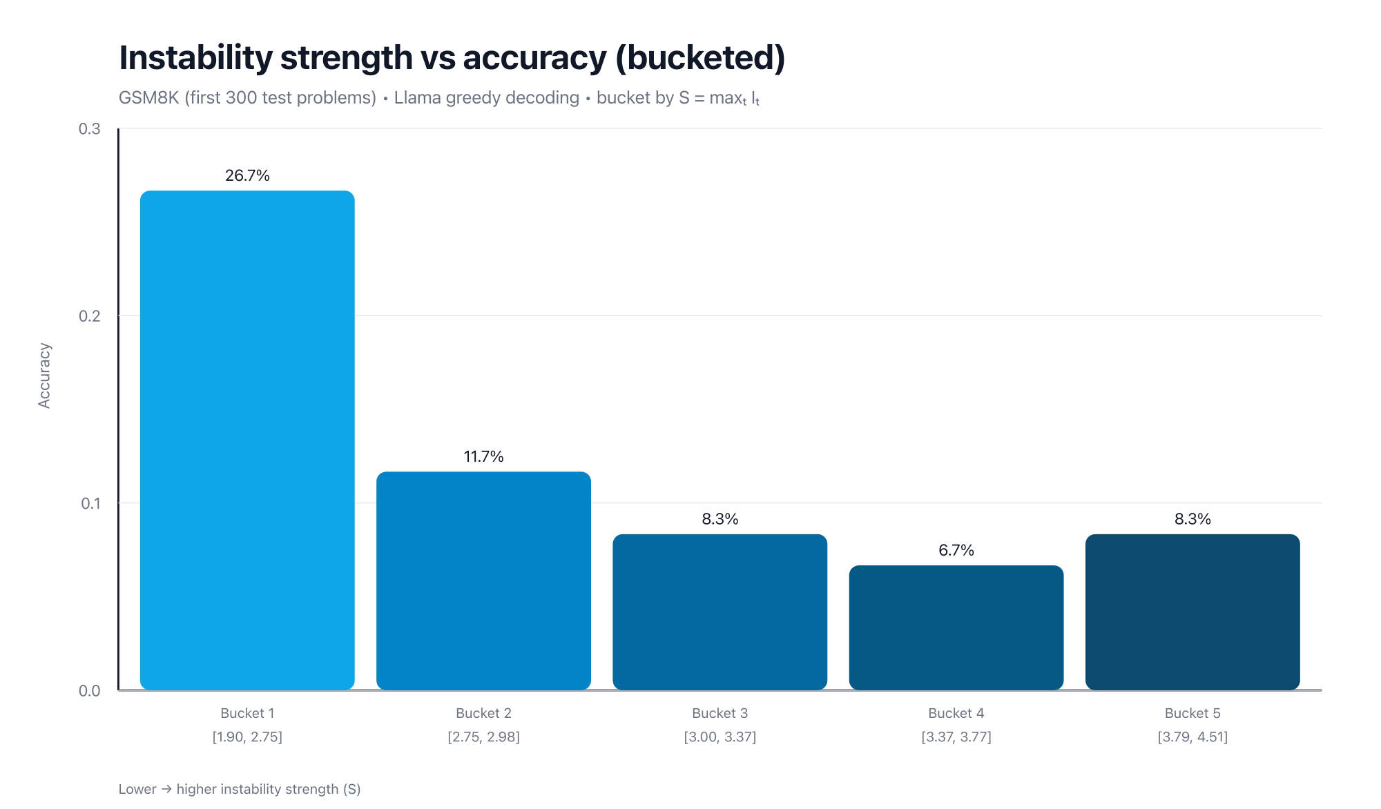
Takeaway:

Higher instability strength corresponds to a higher risk of reasoning failure.

Early warning: you don’t need the whole trace

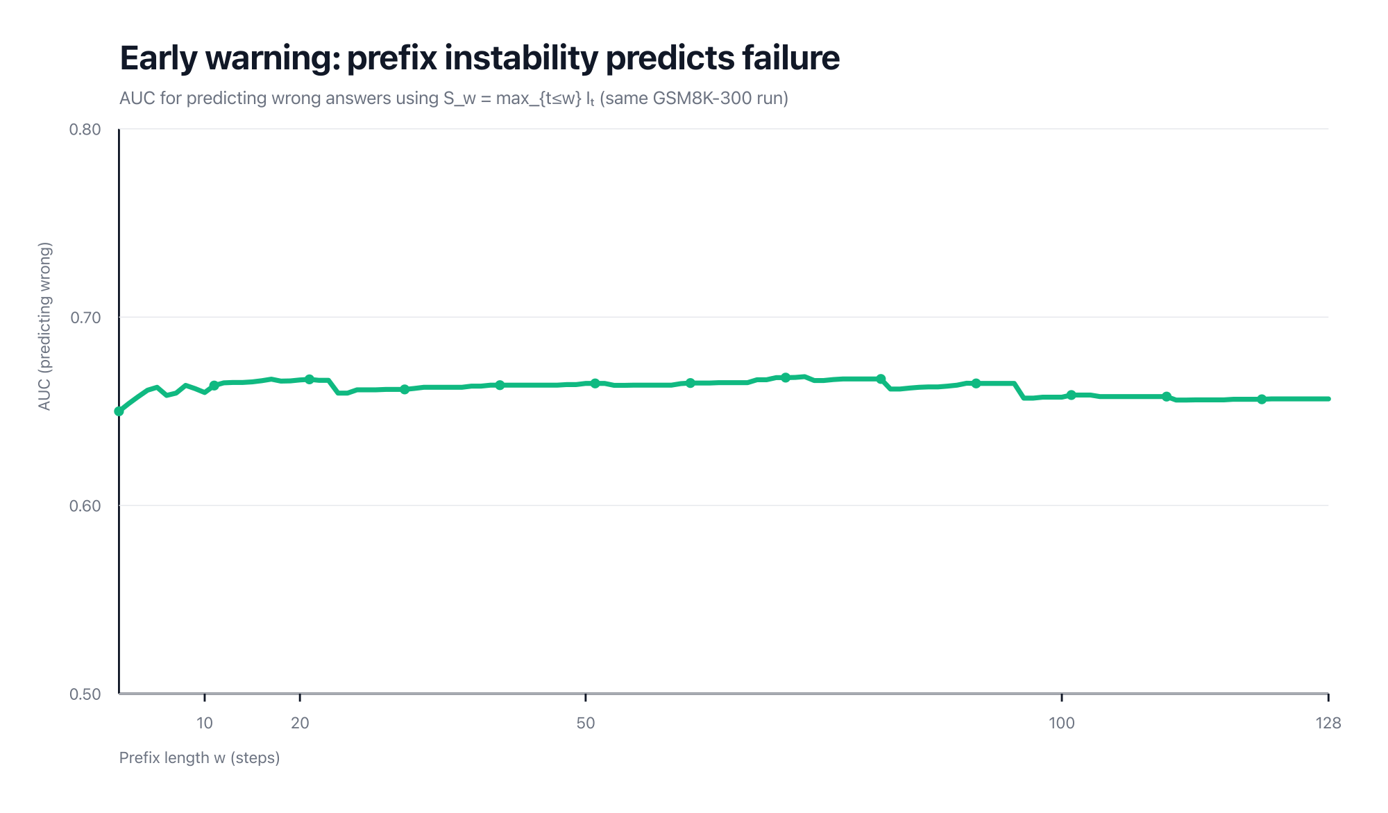
A practical question is whether the signal only appears after the model has already failed.

In the same GSM8K run above, separability is already above chance using short prefixes (e.g., AUC ≈ 0.67 by $w = 20$) and stays roughly stable as we extend the window.

If the curve looks “flat”, that’s the point: most of the separability is already present very early, so additional steps don’t add much extra predictive power (at least under this summary statistic).

Timing matters: corrective vs destructive instability

Here’s the most important nuance:

A high instability spike does not automatically mean “the model is failing.”

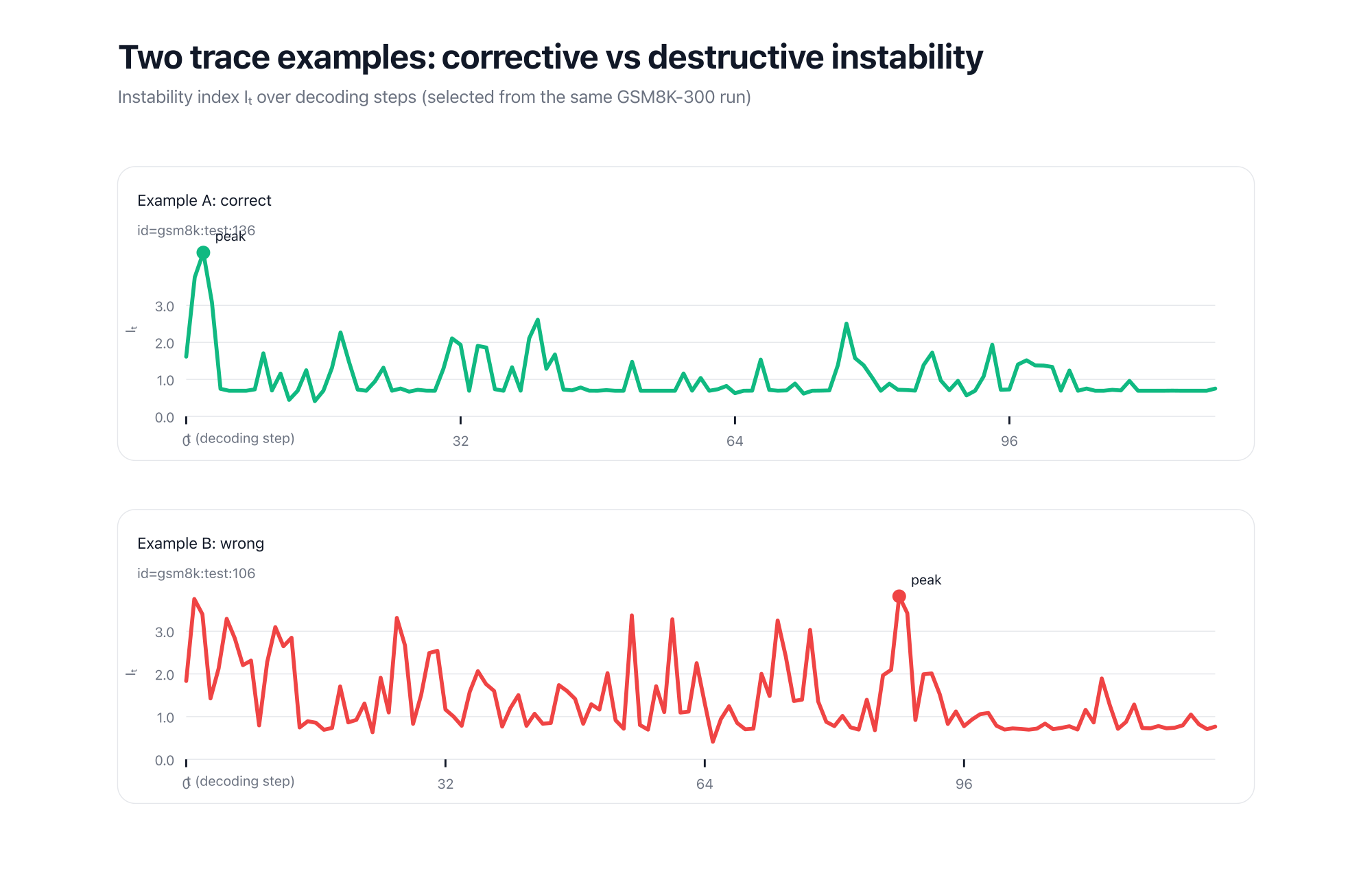
Sometimes, a model becomes briefly unstable because it is self-correcting (switching from a wrong intermediate route to a better one). Other times, instability happens too late, and the model cannot recover.

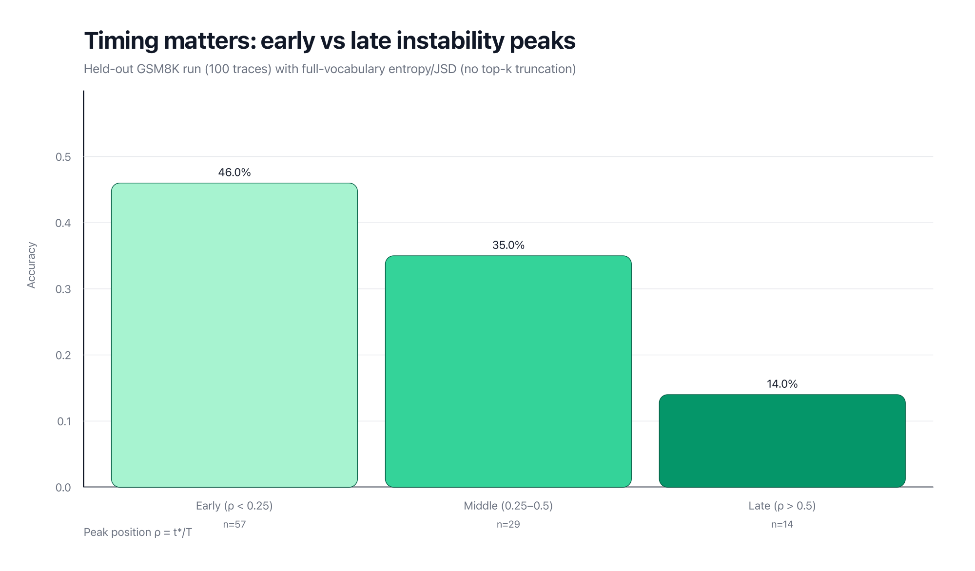
A simple operational proxy is when peak instability occurs.

Let $t^* = \arg\max_t I_t$ be the peak step, $T$ be trace length, and define the relative peak position $\rho = t^*/T$.

• Early peak (small $\rho$): the model has remaining budget to recover.
• Late peak (large $\rho$): there may be no time left to stabilize.

As a sanity check beyond top-$k$ logging, I also ran a small held-out GSM8K set where entropy/JSD are computed from full-vocabulary logits (no truncation). In that run, early-peak traces are much more accurate than late-peak traces (about 46% vs 14%).

To make this concrete, here are two example traces: one correct with an early peak, and one wrong with a late peak.

A small but important limitation: stable-but-wrong failures

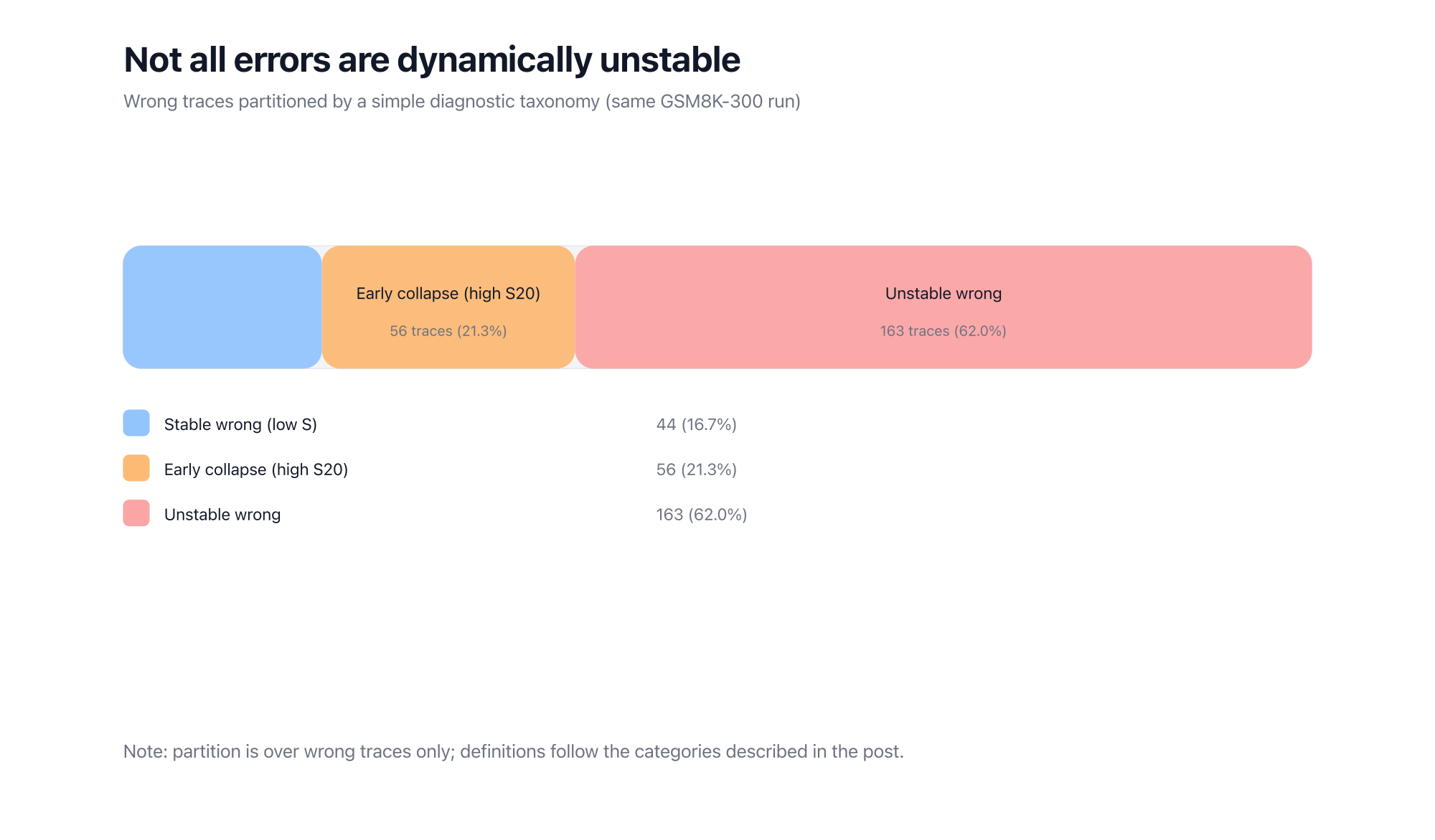
Instability is not a universal explanation of all errors.

Some failures are stable-but-wrong: the model stays confident and consistent, but commits to the wrong solution anyway (knowledge gaps, spurious heuristics, etc.).

This is why I treat instability as a diagnostic dimension, not a catch-all label.

What this diagnostic is (and is not)

What it is:

• A lightweight, inference-time “health monitor” for reasoning trajectories.
• A way to compare models, datasets, and decoding settings by process dynamics, not just accuracy.
• A tool for studying when and how reasoning collapses.

What it is not:

• Not a stabilization method.
• Not an intervention that claims to improve accuracy.

# Inputs: per-step top-k logprobs: logp[t] = {token: log_prob}
# Output: instability strength S

def renormalize(logp_dict):
    # Convert to probabilities and renormalize on logged support
    probs = {tok: math.exp(lp) for tok, lp in logp_dict.items()}
    z = sum(probs.values())
    return {tok: p / z for tok, p in probs.items()}

def entropy(p):
    return -sum(pi * math.log(pi) for pi in p.values() if pi > 0.0)

def jsd(p, q):
    # Compute on union support by zero-padding
    keys = set(p) | set(q)
    m = {k: 0.5 * (p.get(k, 0.0) + q.get(k, 0.0)) for k in keys}
    def kl(a, b):
        return sum(ai * math.log(ai / b[k]) for k, ai in a.items() if ai > 0.0)
    return 0.5 * kl(p, m) + 0.5 * kl(q, m)

p_prev = None
I = []
for t in range(T):
    p_t = renormalize(logp[t])
    H_t = entropy(p_t)
    if p_prev is None:
        D_t = 0.0
    else:
        D_t = jsd(p_t, p_prev)
    I_t = D_t + 1.0 * H_t  # lambda = 1
    I.append(I_t)
    p_prev = p_t

S = max(I)